# init repo notebook
!git clone https://github.com/rramosp/ppdl.git > /dev/null 2> /dev/null
!mv -n ppdl/content/init.py ppdl/content/local . 2> /dev/null
!pip install -r ppdl/content/requirements.txt > /dev/null

Discrete distributions

import numpy as np
from scipy import stats
import matplotlib.pyplot as plt
import pandas as pd
from rlxutils import subplots
import sys
import init
%matplotlib inline

Discrete (or categorical) distributions

we will have a joint distribute distritbution of two variables, in the example below these are \(edad\) and \(barrio\).

• each variable make take any value from a FINITE set. Observe that \(edad\) is discrete because its value comes binned into age groups.

• the possible values for each variable might be sortable in a meaningful way or not. \(edad\) is sortable, \(barrio\) is not, because an alphabetical sorting does not imply any relation.

• for instance, that \(edad\) 10-14 < 25-29 represents a true relation of data (younger/older people)

• but \(barrio\) Aranjuez < Belen does NOT represent any true relation between the two neighborhoods. It is somewhat arbitrary.

recall that:

• the joint probability is the probability of a value of \(edad\) and a value of \(barrio\) for occurring simultaneously. Answers the question: What is the observed proportion of people with age 10-14 and living in Belen.

• the marginal probability is the probability of a value of one variable irrespective of the outcome of the another variable. Answers the question: What is the observed proportion of people living in \(belen\)?.

• the conditional probability is the probability of one event occurring in the presence of a second event. Answers the question: If we only consider people living in \(belen\), what is the observed proportion of people with ages 10-14?

This is the data of people ages and district in Medellin where they live, taken from medata.gov.co

x = pd.read_csv("local/data/proyecciones_de_poblacion_medellin_2017.csv.gz", delimiter=";")
x['grupo_edad'] = x.grupo_edad.str.strip().str.lower()
x = x.rename({"codigo": "barrio", "grupo_edad": "edad"}, axis=1)
x = x.replace("0-4", '00-04').replace('5-9', '05-09').replace('80 y más', '80-')
x = x[x.edad.str.lower().str.strip()!="total"]
x = x[[("Suma" not in i)&("Total" not in i) for i in x.barrio]]
x = x.groupby(["edad", "barrio" ])[['total_2017']].sum().unstack().T.loc['total_2017']

x

edad	00-04	05-09	10-14	15-19	20-24	25-29	30-34	35-39	40-44	45-49	50-54	55-59	60-64	65-69	70-74	75-79	80-
barrio
Altavista	3281	3183	3538	3467	3888	3861	3270	2990	3270	2689	1896	1107	717	520	421	367	109
Aranjuez	10047	10206	10357	10976	11936	13804	13695	11557	9851	11339	12631	11616	8990	6352	4103	2551	2904
Belén	8406	9304	9695	12281	14230	15365	15848	14129	11069	13116	16739	16754	13710	10397	6893	4369	5094
Buenos Aires	6968	7288	7212	8611	10025	11343	11011	9835	8276	9630	11503	11146	8586	6071	3991	2713	3046
Castilla	7844	7986	8228	8743	10642	12446	11560	10021	9083	12129	14627	12250	9130	6665	4253	2652	2622
Doce de Octubre	12714	12562	12473	13301	14749	15935	14512	12670	11435	14508	16409	14151	10555	7568	4926	3150	3169
El Poblado	3666	4212	4527	5353	6363	8189	9540	9600	8681	10461	13356	13622	11246	8634	5739	4086	4211
Guayabal	4175	4428	4523	5268	6217	7460	7620	6692	5463	6768	8231	7821	6743	5364	3552	2546	2526
La América	2439	2883	3034	4091	4923	6154	6775	6377	5143	6418	9502	10146	8779	7678	5315	3393	3868
La Candelaria	3111	3453	3715	4038	4557	6305	7479	6949	5157	5944	7206	7179	6452	5097	3330	2382	3304
Laureles - Estadio	2906	3533	3910	4850	5523	7946	9810	9010	6861	7589	10124	11632	11062	9895	6966	5262	5865
Manrique	11440	11314	11312	11756	12422	13701	12536	10458	9325	11208	12622	11293	8057	5460	3568	2238	2360
Palmitas	474	417	543	609	666	646	505	430	634	611	507	361	233	198	109	87	31
Popular	11799	11707	11113	11056	10779	10956	10037	8971	7859	8280	8382	6789	4860	3426	2228	1589	1614
Robledo	10897	11153	11142	12065	13989	14847	13997	12195	10244	11809	13580	12245	9498	6923	4467	2596	2759
San Antonio	8610	8208	9796	9925	11907	11737	10736	9990	11105	8874	6166	4119	2517	1601	1102	875	326
San Cristóbal	6985	6898	8400	8337	9241	9375	8014	7614	8303	6913	4641	3257	1901	1243	887	780	283
San Javier	9775	10642	10930	11672	11885	12005	11317	10307	8614	8838	9205	7705	5679	4049	2620	1693	2239
Santa Cruz	8789	8720	8546	8891	9289	9814	9039	7867	6491	7037	7978	6554	4581	3424	2257	1471	1766
Santa Elena	1559	1491	1725	1670	1785	1997	1757	1495	1514	1488	1077	678	511	353	250	159	50
Villa Hermosa	9971	10346	10228	11280	11901	12581	11909	10075	7885	7939	8694	7737	6052	4552	2970	1952	2470

joint distribution

we turn it into a joint distribution. This is an empirical distribution, because the data was obtained by counting using some method on the real world and not derived or assumed by some analytical procedure or calculation.

xd = x/x.values.sum()
xd

edad	00-04	05-09	10-14	15-19	20-24	25-29	30-34	35-39	40-44	45-49	50-54	55-59	60-64	65-69	70-74	75-79	80-
barrio
Altavista	0.001308	0.001269	0.001410	0.001382	0.001550	0.001539	0.001304	0.001192	0.001304	0.001072	0.000756	0.000441	0.000286	0.000207	0.000168	0.000146	0.000043
Aranjuez	0.004005	0.004069	0.004129	0.004376	0.004758	0.005503	0.005460	0.004607	0.003927	0.004520	0.005035	0.004631	0.003584	0.002532	0.001636	0.001017	0.001158
Belén	0.003351	0.003709	0.003865	0.004896	0.005673	0.006125	0.006318	0.005633	0.004413	0.005229	0.006673	0.006679	0.005466	0.004145	0.002748	0.001742	0.002031
Buenos Aires	0.002778	0.002905	0.002875	0.003433	0.003996	0.004522	0.004390	0.003921	0.003299	0.003839	0.004586	0.004443	0.003423	0.002420	0.001591	0.001082	0.001214
Castilla	0.003127	0.003184	0.003280	0.003485	0.004242	0.004962	0.004608	0.003995	0.003621	0.004835	0.005831	0.004883	0.003640	0.002657	0.001695	0.001057	0.001045
Doce de Octubre	0.005068	0.005008	0.004972	0.005302	0.005880	0.006353	0.005785	0.005051	0.004559	0.005784	0.006541	0.005641	0.004208	0.003017	0.001964	0.001256	0.001263
El Poblado	0.001461	0.001679	0.001805	0.002134	0.002537	0.003265	0.003803	0.003827	0.003461	0.004170	0.005324	0.005430	0.004483	0.003442	0.002288	0.001629	0.001679
Guayabal	0.001664	0.001765	0.001803	0.002100	0.002478	0.002974	0.003038	0.002668	0.002178	0.002698	0.003281	0.003118	0.002688	0.002138	0.001416	0.001015	0.001007
La América	0.000972	0.001149	0.001210	0.001631	0.001963	0.002453	0.002701	0.002542	0.002050	0.002559	0.003788	0.004045	0.003500	0.003061	0.002119	0.001353	0.001542
La Candelaria	0.001240	0.001377	0.001481	0.001610	0.001817	0.002514	0.002982	0.002770	0.002056	0.002370	0.002873	0.002862	0.002572	0.002032	0.001328	0.000950	0.001317
Laureles - Estadio	0.001158	0.001408	0.001559	0.001933	0.002202	0.003168	0.003911	0.003592	0.002735	0.003025	0.004036	0.004637	0.004410	0.003945	0.002777	0.002098	0.002338
Manrique	0.004561	0.004510	0.004510	0.004687	0.004952	0.005462	0.004998	0.004169	0.003717	0.004468	0.005032	0.004502	0.003212	0.002177	0.001422	0.000892	0.000941
Palmitas	0.000189	0.000166	0.000216	0.000243	0.000266	0.000258	0.000201	0.000171	0.000253	0.000244	0.000202	0.000144	0.000093	0.000079	0.000043	0.000035	0.000012
Popular	0.004704	0.004667	0.004430	0.004407	0.004297	0.004368	0.004001	0.003576	0.003133	0.003301	0.003342	0.002706	0.001937	0.001366	0.000888	0.000633	0.000643
Robledo	0.004344	0.004446	0.004442	0.004810	0.005577	0.005919	0.005580	0.004862	0.004084	0.004708	0.005414	0.004881	0.003786	0.002760	0.001781	0.001035	0.001100
San Antonio	0.003432	0.003272	0.003905	0.003957	0.004747	0.004679	0.004280	0.003983	0.004427	0.003538	0.002458	0.001642	0.001003	0.000638	0.000439	0.000349	0.000130
San Cristóbal	0.002785	0.002750	0.003349	0.003324	0.003684	0.003737	0.003195	0.003035	0.003310	0.002756	0.001850	0.001298	0.000758	0.000496	0.000354	0.000311	0.000113
San Javier	0.003897	0.004242	0.004357	0.004653	0.004738	0.004786	0.004512	0.004109	0.003434	0.003523	0.003670	0.003072	0.002264	0.001614	0.001044	0.000675	0.000893
Santa Cruz	0.003504	0.003476	0.003407	0.003544	0.003703	0.003912	0.003603	0.003136	0.002588	0.002805	0.003180	0.002613	0.001826	0.001365	0.000900	0.000586	0.000704
Santa Elena	0.000621	0.000594	0.000688	0.000666	0.000712	0.000796	0.000700	0.000596	0.000604	0.000593	0.000429	0.000270	0.000204	0.000141	0.000100	0.000063	0.000020
Villa Hermosa	0.003975	0.004124	0.004077	0.004497	0.004744	0.005015	0.004748	0.004016	0.003143	0.003165	0.003466	0.003084	0.002413	0.001815	0.001184	0.000778	0.000985

# it must add up to 1
xd.values.sum()

1.0

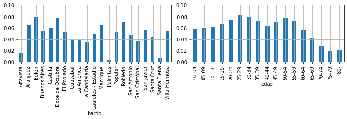
marginal distribution

This are the TWO marginal distributions, for each one of the variables

dbarrio = xd.sum(axis=1)
dedad   = xd.sum(axis=0)

dbarrio.sum(), dedad.sum()

(1.0, 1.0)

for ax,i in subplots(2, usizex=5, usizey=3.5):
    if i==0: dbarrio.plot(kind="bar")
    if i==1: dedad.plot(kind="bar")
    plt.grid()
    plt.ylim(0,0.1)
plt.tight_layout()
        

conditional distribution

we compute it for one variable with respect to a specific value of the other one.

This is

\[P(\text{edad}|\text{barrio}=\text{belen})\]

observe that we obtain it from the join distribution but WE MUST NORMALIZE so we have a true distribution adding up to 1.

This normalization will become very important later on in the course.

# unnormalized conditional

xd.loc['Belén']

edad
00-04    0.003351
05-09    0.003709
10-14    0.003865
15-19    0.004896
20-24    0.005673
25-29    0.006125
30-34    0.006318
35-39    0.005633
40-44    0.004413
45-49    0.005229
50-54    0.006673
55-59    0.006679
60-64    0.005466
65-69    0.004145
70-74    0.002748
75-79    0.001742
80-      0.002031
Name: Belén, dtype: float64

# it does not add up to one
xd.loc['Belén'].sum()

0.07869355283657012

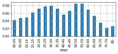
# we normalized it

dbelen = xd.loc['Belén'] / xd.loc['Belén'].sum()
print ("check sum =", dbelen.sum())
dbelen

check sum = 1.0

edad
00-04    0.042584
05-09    0.047133
10-14    0.049114
15-19    0.062214
20-24    0.072087
25-29    0.077837
30-34    0.080284
35-39    0.071576
40-44    0.056074
45-49    0.066444
50-54    0.084798
55-59    0.084874
60-64    0.069453
65-69    0.052670
70-74    0.034919
75-79    0.022133
80-      0.025806
Name: Belén, dtype: float64

dbelen.plot(kind='bar', figsize=(6,2))
plt.grid();

Sometimes we write

\[P(\text{edad}|\text{barrio})\]

without specifying the value of the conditioning variable, but assuming someone has decided upon a certain value. You must pay attention to the context in which this is being used to understand well how to compute or use this conditional distribution.

In fact, for each value of \(barrio\) we have a different distritbuion.

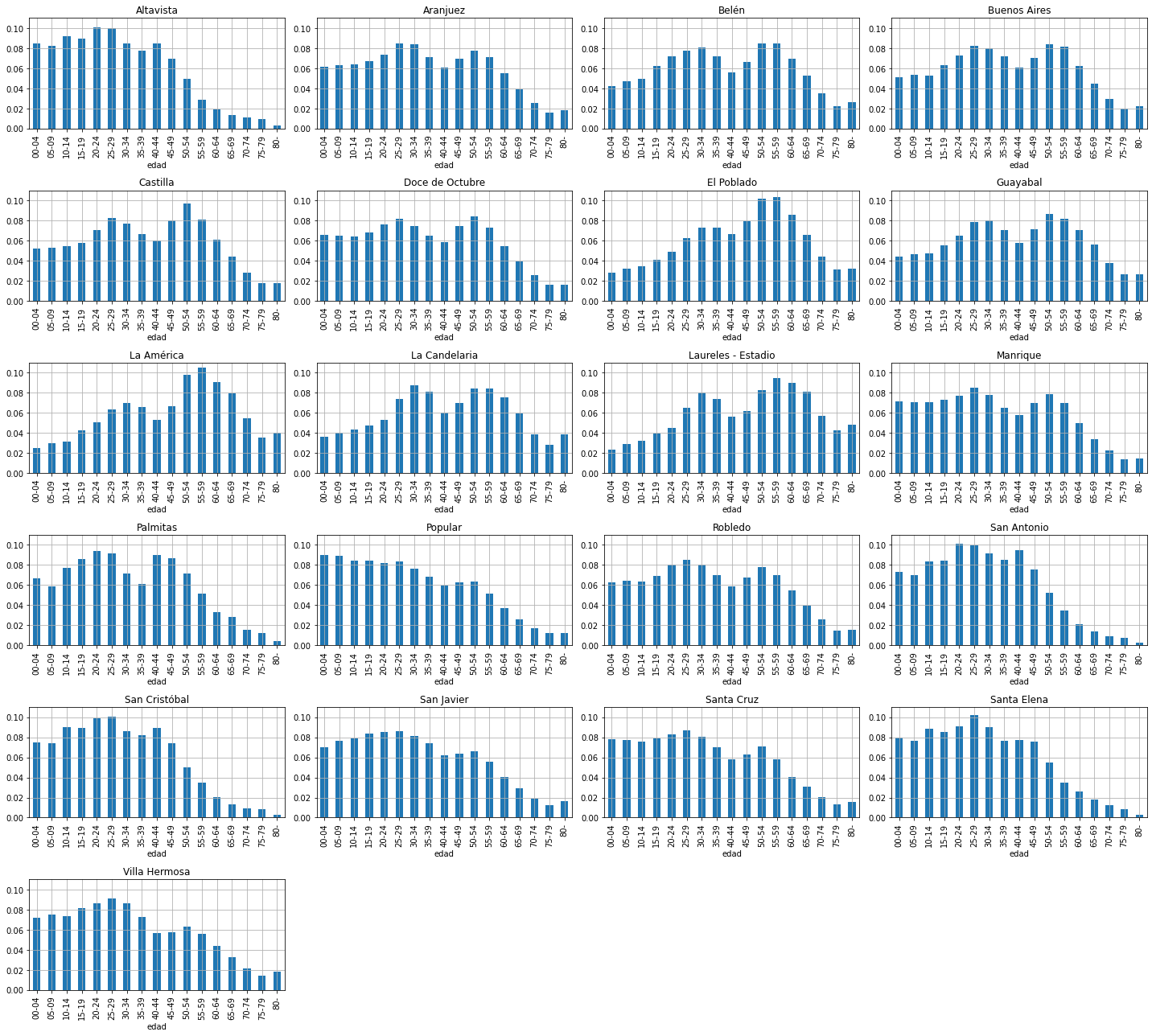
independance

Observe carefully. If all conditional distributions look the same this suggests that both variables are independant, \(\rightarrow\) knowing something about one does not tell us anything about the other one.

for ax,barrio in subplots(xd.index, usizex=5, usizey=3, n_cols=4):
    dmarginal = xd.loc[barrio] / xd.loc[barrio].sum()
    dmarginal.plot(kind='bar', ax=ax)
    plt.title(barrio)
    plt.ylim(0,.11)
    plt.grid();
plt.tight_layout()

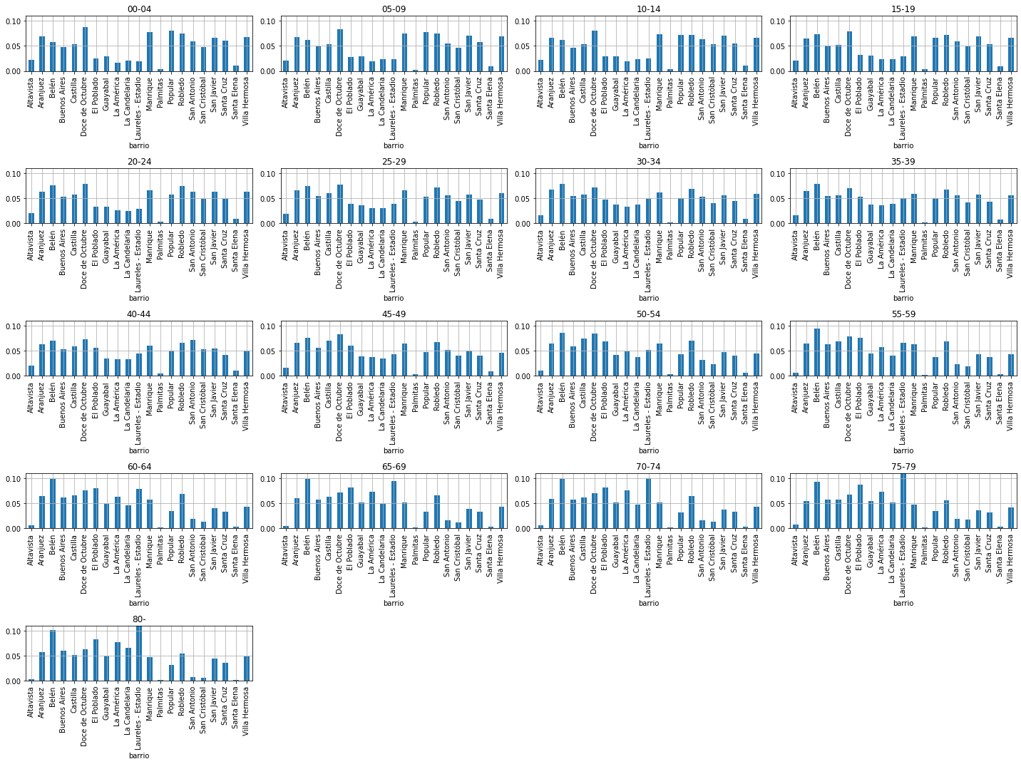
or for each value of \(edad\)

for ax,edad in subplots(xd.columns, usizex=5, usizey=3, n_cols=4):
    dmarginal = xd[edad] / xd[edad].sum()
    dmarginal.plot(kind='bar', ax=ax)
    plt.title(edad)
    plt.ylim(0,.11)
    plt.grid();
plt.tight_layout()